Inferring budding phylogenetic trees with the stratigraphic-range fossilized birth-death model

Introduction

Overview

In this tutorial, we will use cutting-edge fossil-phylogenetic methods to estimate trees with oriented (i.e. budding) speciation nodes. These trees also explicitly accommodate stratigraphic ranges (the time between first and last occurrence of a species), allowing for a more taxonomic approach that better matches the assumptions of the fossil record. In particular, we will use the stratigraphic-range fossilized birth-death model (SRFBD) (Stadler et al. (2018), Stolz et al. (2025)), which expands on the FBD model (Stadler (2010), Heath et al. (2014)) to allow for stratigraphic ranges and budding speciation. This model is most appropriate for groups with a dense fossil record with multiple specimens per species.

To illustrate its benefits, we will be using the Canidae dataset first published by Slater (2015), later complemented with some extra data for a test of the SRFBD implementation in Stolz et al. (2025). This dataset contains 116 extinct and 5 extant canid species, including stratigraphic ranges (times of first and last fossil occurrence), and morphological characters (123 characters, including 2, 3, 4, and 5 state characters). We will then use R to analyze the results of the SRFBD analysis, and gain some insight on what budding phylogenetic trees can tell us about the evolutionary history of canids.

Getting Started

If you’d prefer to follow this tutorial through an R markdown file, download it here:

srfbd.Rmd

Once you’ve installed the required software and downloaded all the files above, let’s start setting up our analyses. First, make sure to add all the files to some directory–that will be our working directory. I like to organize things into data, scripts, and output directories, but feel free to organize it differently if it makes more sense to you!

For me, I have a directory within my website called srfbd, and within it I have a data directory with the morphological and range data files, and a scripts directory where we will be writing all of our BEAST2 scripts. The two xml template files and R script writing files provided with this tutorial are on the srfbd directory itself. Let’s set up some useful directory variables!

# base directory, where your .xml and .R files are
base_dir <- "/Users/petrucci/Documents/website/brpetrucci.github.io/files/tutorials/srfbd/"

# scripts, data, and output directories
scripts_dir <- paste0(base_dir, "scripts/")
data_dir <- paste0(base_dir, "data/")
out_dir <- paste0(base_dir, "output/")

We will use these directories to write our scripts, and then analyze the output later. Of course you could simply

You also need to install and attach the packages discussed above.

# install packages from CRAN
install.packages(c("ape", "coda", "devtools"))

# install the paleobuddy development branch
pak::pak("brpetrucci/paleobuddy@development")

We can then attach them.

# attach packages
library(ape)
library(coda)
library(paleobuddy)

We are now ready to start the tutorial proper!

Inference

Writing scripts

First, let’s write some BEAST2 scripts! Because there is currently no available BEAUti template for the SRFBD model, we must do some manual writing, which is challenging for xml files. The usual process would be writing a template with BEAUti for a traditional FBD analysis, then careful reading of a working SRFBD xml to apply all the required changes. It’s a lengthy and error-prone process, especially if you’re not used to the xml format. Lucky for you, I suffered so you don’t need to! I wrote a few scripts to do the process for you. Here’s a rundown:

• xml_writer.R creates a ton of functions that write the script proper. It reads the user’s preferences (laid out in canidae_setup.R or a file like it) and writes each part of the xml for a complete SRFBD analysis. It is certainly not encompassing of all the possible variation you could have in an SRFBD analysis, however–only the specifics I have needed for my analyses in the past. Please feel free to contact me for any help modifying this (and any other file in this tutorial) for your uses.
• canidae_setup.R sets up the specifics we would like for the Canidae analysis, through writing one simple function: scripts_setup(). That function is where you would set your data, priors, and operators. It is currently set up for the simple morphological-only analysis we will use as an example in this tutorial, but xml_writer.R is perfectly able to handle DNA data as well, and all one would need to add molecular data into the mix is to create analogous priors, operators, and data blocks to the morphological ones here. Similarly, any modifications to the desired specifications (e.g., using a different morphological clock model) would be achievable by slightly changing (or adding/removing) the priors and operators. It is difficult to give a full rundown of these scripts in a short tutorial, but they have hopefully been commented enough for understanding. In the future I will add more setup scripts to show examples of how we might set up different analyses.
• header.xml and maps.xml are simple templates needed for the xml file, that are too long to justify writing into an R string. Simply keep them in the same base_dir as the R files and you should not have to worry about them.

Now let’s write some xml scripts! Here we need to consider a few questions about our MCMC setup, which I set as arguments for the scripts_setup function.

• n_scripts describes how many scripts we would like to build with the exact same setup. Running multiple analyses for the same script is recommended so you can ensure your final posterior sample is not affected by the initial state. For your convenience, xml_writer.R automatically chooses new initial states (drawing each initial value from the corresponding prior) each time it writes a new script, so you just need to tell it how many scripts to write. I chose 4, but feel free to run more or less depending on the resources you have available.
• n_gens describes how many generations we should run our MCMC for. I am using 1 billion generations, which is likely overkill for a morphological-only model. Again, feel free to change this value. BEAST2 makes it very easy to resume runs if you feel like it needs more generations, so don’t feel stressed about this choice.
• log_every describes how often we want the model to sample from the MCMC and store the current values of our parameters and tree in the corresponding .log and .trees files. I set it to 1 million, so that each run will end with 1000 posterior samples before burnin.
• store_every describes how often BEAST2 should store the current value of parameters in a .state file, which can then be used to resume analyses. I recommend setting this to the same value as log_every, so as to avoid jumps in your posterior sample in case you need to resume an analysis. For more details on resuming an analysis, check out the Resuming BEAST2 runs box below.
• attach describes where in the stratigraphic range of each species to attach the morphological data. One might choose to attach the data at both the first and last occurrence ("both"), or just the first occurrence ("first"). It is unclear as of now which of the two approaches lead to more accurate estimates (I’m working on it!), but for the sake of example here we will just attach the data to the first occurrence.

Now that we understand the arguments, we just need to source the setup scripts, set values for the arguments, and run the scripts_setup function!

# source your setup script
source(paste0(base_dir, "canidae_setup.R"))
# xml_writer.R is already sourced by the setup script

# number of scripts
n_scripts <- 4

# number of generations
n_gens <- 1000000000

# how often to sample the MCMC and store into .log and .trees files
log_every <- 1000000

# how often to store the current state into .state file
store_every <- 1000000

# which occurrence do we want to attach the morphological data to?
attach <- "first"

# write scripts
scripts_setup(n_scripts, n_gens, attach, 
              scripts_dir, log_every, store_every)

This will write scripts of the form srfbd_first_N.xml into the scripts/ directory, where N goes from 1 to n_scripts (the _N is ommitted if you choose to set n_scripts to 1). Feel free to alter the script_name variable in canidae_setup.R to change that convention.

Running the Analysis

Now that we have our scripts ready, let’s run them! You can of course do all of the steps I will list below using the GUIs installed with BEAST2 in your local machine. This would take quite a bit of time though, so I will assume you are running these commands on a cluster, and will therefore list command line commands for them.

First, we need to run our BEAST2 analyses proper. Again I will assume you have your scripts in the scripts directory, and a (currently empty) output directory in the same parent folder. For each script script/script.xml, we can run:

/path/to/beast/bin/beast scripts/script.xml

By default, the beast executable will be installed to the bin directory of the overarching beast installation folder. In my cluster, the first command reads /home/petrucci/beast/bin/beast, for example. Of course if you’d prefer you could add the bin directory to your PATH in order to be able to just use the beast command.

If you build your scripts using my canidae_setup.R script as-is, this analysis will write your output files as output/script.log and output/script.trees. You may change this in the <logger fields within xml_writer.R, if you choose.

/path/to/beast/bin/beast -resume scripts/script.xml

Once your analyses are done running (they took 2-4 days in my cluster, but that might vary), we then need to test them for convergence, and combine them into one aggregate posterior sample. Optionally, you might also want to obtain a summary tree for your analysis. Let’s go through the commands for each of these steps below.

First, let’s test convergence. Most researchers would use the Tracer software for this, and BEAST2 has a great tutorial for doing just that. I recommend you check your output with Tracer, but here I will present an alternative way to check convergence using the R package coda.

We will read each of our log files into R, use coda to check their effective sample size (ESS) with effectiveSize, and ensure we have a good effective sample size for each of them. We will apply a 50% burnin, but feel free to check how things change by changing the burnin argument below.

# burnin percentage
burnin <- 0.5

# number of columns in your log (excluding sample column)
n_cols <- 23
# make sure to change this if you are running this for your
# own analysis and have a different number of parameters

# data frame to hold our effective sample sizes
ess_df <- data.frame(matrix(nrow = n_scripts, ncol = n_cols))

# iterate through our scripts
for (i in 1:n_scripts) {
  # read this log
  log <- read.delim(paste0(out_dir, "srfbd_first_", i, ".log"),
                    sep = "\t", header = TRUE, comment.char = "#")
  # the comment.char argument is needed because BEAST2
  # writes the entire script to the top of the log file,
  # but we can ignore that with comment.char
  
  # we need to remove the first column, since that's just the generation marker
  log <- log[, -1]
  
  # then we need to apply some burnin
  log <- log[(0.5 * nrow(log) + 1):nrow(log), ]
  # this will leave us with 500 samples per log
  # the +1 is required since BEAST2 records the initial state
  
  # finally, we can use coda to check the effective sample size
  ess <- coda::effectiveSize(log)
  
  # add to our data frame
  ess_df[i, ] <- ess
}

# name ess_df columns
colnames(ess_df) <- colnames(log)

# check the minimum
unlist(sapply(1:ncol(ess_df), function(c) min(ess_df[, c])))

##  [1] 244.4926 280.4763 174.1771 325.4456 500.0000 258.4932 500.0000 435.0881 184.8303 337.4784 397.8647 312.5460
## [13] 500.0000 500.0000 500.0000 327.4611 400.9191 293.6815 401.8065 408.8584 171.7148 399.0280 344.5501

For my analyses, the lowest ESS was ~171, which is pretty good. coda uses a bit of a stricter calculation for ESS than Tracer, so do not be surprised if you see higher values in that software. Since we have achieved convergence in each of our runs, we can then use the BEAST2 companion program LogCombiner to aggregate our posterior samples into one.

/path/to/beast/bin/logcombiner -b 50 \
-log output/srfbd_first_1.log \
-log output/srfbd_first_2.log \
-log output/srfbd_first_3.log \
-log output/srfbd_first_4.log \
-o output/srfbd_first.log

/path/to/beast/bin/logcombiner -b 50 \
-log output/srfbd_first_1.trees \
-log output/srfbd_first_2.trees \
-log output/srfbd_first_3.trees \
-log output/srfbd_first_4.trees \
-o output/srfbd_first.trees        

You may then do your due diligence and check that the srfbd_first.log file also shows we have converged. This is necessary because even if all four of our separate scripts have converged, they might have converged to different parameter values. Checking this final file for convergence would of course be a straightforward exercise of repeating your coda or Tracer checks above, so I will leave that to you.

Now that we have our final log and tree files, each with around 2000 samples, we can proceed to analyze our results. First, however, you might want to generate a tree summary. While a thorough examination of your full posterior sample is of course necessary for any Bayesian analysis, it is often difficult to avoid the generation of a tree summary. You might need one tree to run some comparative methods on, or simply would like to have a representative tree to add to your paper/talk.

Since SRFBD generates budding phylogenetic trees, building tree summaries is also something we need new tools for. The sRanges package already contains an implementation of a maximum clade-credibility (MCC) tree algorithm. Let’s build our tree and see how it looks! Note that we will need the SRTreeAnnotator tool for this, which requires applauncher (accessible in BEAUti through File > Launch apps, if you’d like a GUI).

/path/to/beast/bin/applauncher SRTreeAnnotator -burnin 0 \
-trees output/srfbd_first.trees \
-out output/srfbd_first_mcc.nex

While paleobuddy does include functions to plot a budding phylogeny, the R plotting window is not ideal for visualizing phylogenies with more than a few dozen tips. Luckily, IcyTree is a very powerful browser-based tool for visualizing trees, and it already allows for the visualization of budding phylogenies. Simply select the srfbd_first_mcc.nex file, then click Style > Tree layout > Transmission tree. You can visualize the stratigraphic ranges of each species by selecting Style > Colour edges by > range, and mark sampled ancestors (fossil samples that left sampled descendants, i.e. fossils that are not tips) by pressing m. Feel free to play around with other style options–IcyTree is a great tool for generating publication-level images of phylogenies, even budding ones!! Let’s see how our tree turned out.

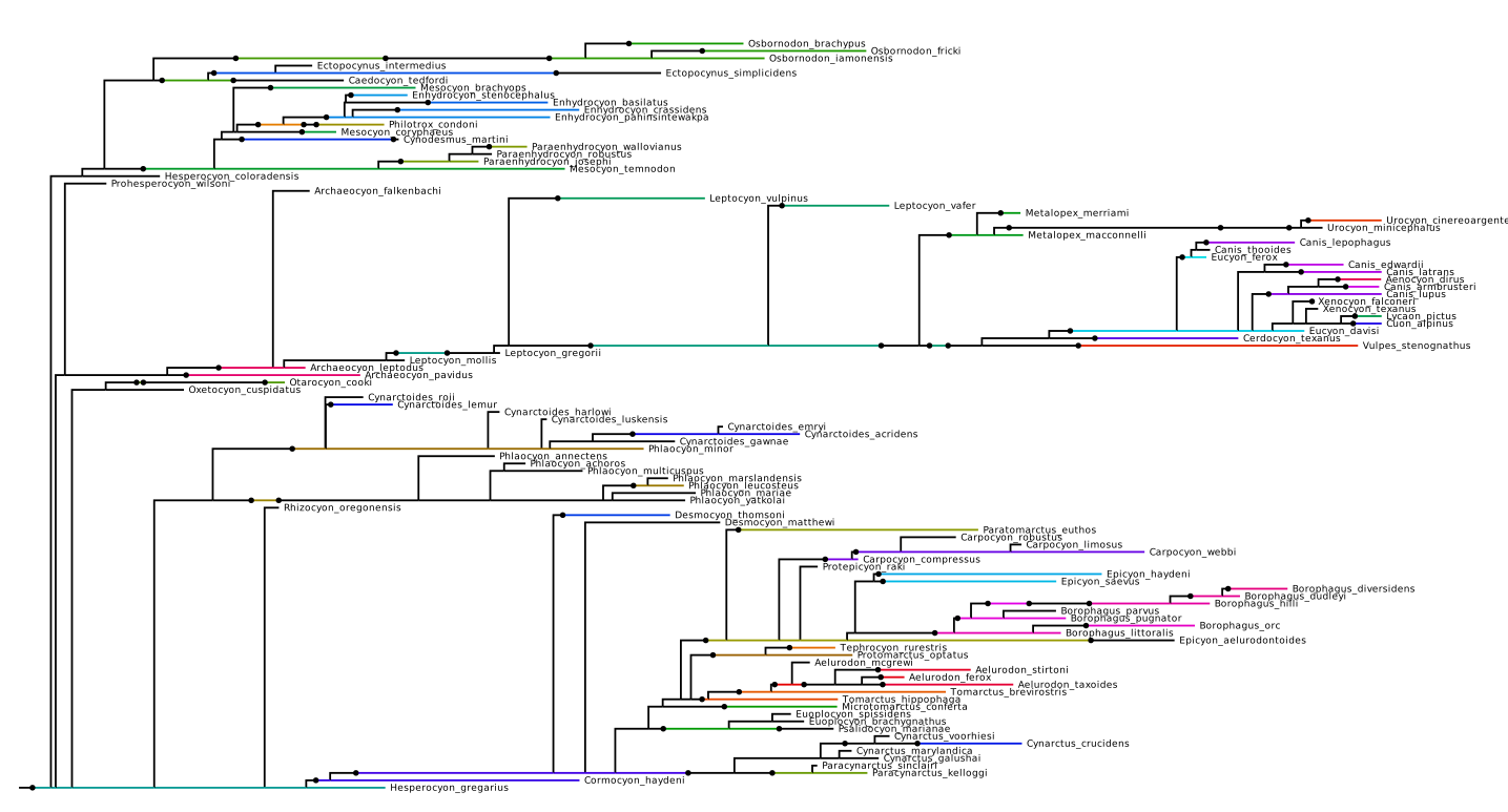I made the font for the species names reasonably small because they start overlapping each other, but you can zoom in on your own tree to explore the topology in more detail. Note that by default the tips will be called genus_species_last or genus_species_first, since they represent a first/last occurrence rather than a species. If you’d like to label them by species, select Style > Tip text > taxon.

One thing to note about the trees we get as output from SRFBD is that besides being budding trees, they also maintain the taxonomic continuum implied by stratigraphic ranges. That means any tree that would break an SR (i.e. placing the genus_species_first and genus_species_last in separate branches of the tree) would not be accepted by the model, so you can be sure that every SR tree (as we have come to call these) will have the SR of a species as one unbroken segment within a branch.

We will discuss the MCC tree further in our results below, so keep it in your back pocket! In case you haven’t had time to run the full analysis yet but want to run our results, you can download the result files from my analysis:

Log file Tree file (compressed) MCC tree

Results

Parameter estimates

To start, we can take a look at the diversification and fossil sampling rate estimates from our model. While this is a constant-rate model, and therefore not incredibly realistic (keep an eye on Kate Truman from the Gavryushkina lab for a paper on the skyline SRFBD model coming out soon!), this is still a worthy exercise.

# read the full log
log <- read.delim(paste0(out_dir, "srfbd_first.log"), 
                  sep = "\t", header = TRUE, comment.char = "#")[, -1]

# let's check the histograms for our rates and origin
par(mfrow = c(2, 2))

# sampling proportion
hist(log$samplingProportionFBD, 
     main = "Posterior sample of sampling proportion",
     xlab = "diversification (proportion of species)",
     probability = TRUE)
abline(v = mean(log$samplingProportionFBD), col = "#DF536B", lwd = 2)
curve(dbeta(x, 3.1, 6.9), add = TRUE, col = "#2297E6", lwd = 2)

# let's look at the 95% credible interval for this one
quantile(log$samplingProportionFBD, c(0.025, 0.975))

##      2.5%     97.5% 
## 0.5806821 0.7135636

# diversification rate
hist(log$diversificationRateFBD, 
     main = "Posterior sample of diversification rate",
     xlab = "diversification (events/lineage/my)",
     probability = TRUE)
abline(v = mean(log$diversificationRateFBD), col = "#DF536B", lwd = 2)
curve(dexp(x, 1 / 0.0767), add = TRUE, col = "#2297E6", lwd = 2)

# turnover
hist(log$turnoverFBD, 
     main = "Posterior sample of turnover",
     xlab = "turnover",
     probability = TRUE)
abline(v = mean(log$turnoverFBD), col = "#DF536B", lwd = 2)
curve(dbeta(x, 2, 1), add = TRUE, col = "#2297E6", lwd = 2)

# origin
hist(log$originFBD, 
     main = "Posterior sample of the origin",
     xlab = "origin (mya)",
     probability = TRUE)
abline(v = mean(log$originFBD), col = "#DF536B", lwd = 2)
curve(dexp(x - 37, 1 / 9.67), add = TRUE, col = "#2297E6", lwd = 2)

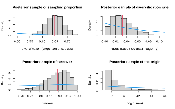
To better visualize things, I added a red line marking the posterior mean, and a blue line showing the prior distribution. You can see that for every parameter we’ve checked, the posterior sample is pretty different from the prior, which is a good sign! It is an indication that our results are coming from the data, as opposed to just returning the prior (which might happen when your data are not very informative).

What we see for diversification and turnover is pretty standard: low diversification, turnover very close to 1. This is why skyline models are useful–if we are just trying to fit one rate to an entire tree, we end up on an average that just relates to the general trend of going from one species to a few in ~40 million years. For example, the maximum likelihood estimate for diversification rate for a tree with 5 extant species that started at time $T$ with one species is $ln(5) / T$. If we took $T = 38$ that’s around $0.04$, which is pretty close to our posterior sample. Still, it is good to see that the results make sense.

For our sampling proportion, we see a mean of $0.65$, with a 95% credible interval of ${0.59, 0.71}$. This indicates an estimate of 178-215 total extinct canid species. By my estimations there are 206 described extinct canids, and while this number will change with which expert you consult (and, more importantly, there is an unknown number of undescribed ones), the model estimates seem reasonable.

Finally, let’s talk about the origin. Our prior distribution (an exponential with an offset of $37$mya and rate of $9.67$) was chosen because it has a minimum around the oldest possible fossil occurrence in our dataset, 95% of the density below 66mya (around the K-Pg boundary), and a mean of around $47$mya, which is the age of some basal caniforms. Our posterior sample seems to indicate a lot of confidence that the origin is on the lower range of that, closer to $37$mya.

While the rates estimated by SRFBD are easy to interpret, it is occasionally useful to reparameterize the rates to speciation, extinction, and fossil sampling.

# do the transformations backwards
lambda <- log$diversificationRateFBD / (1 - log$turnoverFBD)
mu <- lambda * log$turnoverFBD
psi <- log$samplingProportionFBD * mu / (1 - log$samplingProportionFBD)

# plot the histograms
par(mfrow = c(3, 1))
hist(lambda, 
     main = "Posterior sample of speciation rate",
     xlab = "speciation rate (events/lineage/my)",
     probability = TRUE)
hist(mu, 
     main = "Posterior sample of extinction rate",
     xlab = "extinction rate (events/lineage/my)",
     probability = TRUE)
hist(psi, 
     main = "Posterior sample of fossil sampling rate",
     xlab = "fossil sampling rate (events/lineage/my)",
     probability = TRUE)

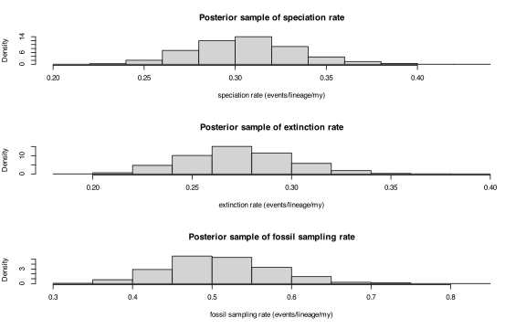
It seems like we would expect, on average, a speciation event every ~3my, an extinction event every ~4my, and a sampling event every ~2my, per living lineage. Again, not much of interest to explore without skyline rates, but just an illustration of what we could explore with rate estimates.

One last interesting parameter to explore here is the sampled ancestor counts. Sampled ancestors represent hidden speciation events, i.e. when a species might have generated a different species after the time of its last fossil sample. They might also be the signature of anagenesis, and it might be impossible to distinguish between these two possibilities. Either way, the number of species estimated to be sampled ancestors may be of interest.

# histogram of the number of sampled ancestors
hist(log$SACountFBD, 
     main = "Posterior sample of sampled ancestor count",
     xlab = "Number of sampled ancestor species")

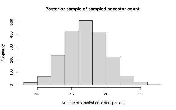
It seems like we have a median of around 17 species being sampled ancestors, which is reasonably low (14%). In my tests of SRFBD and traditional FBD (in prep), I’ve found that SRFBD is generally more conservative in setting species as sampled ancestors, which leads it on average to miss some SAs, but have a reasonable degree of confidence in the species it does assign as SAs being SAs. We will keep this in mind in our discussion of topology below.

We could also spend some time looking at our morphological evolution parameter estimates, but will skip that to avoid making a long tutorial even longer. In a future tutorial I mean to explore how the choice of where to place our data (first occurence or both first and last occurrence) may change our results.

Phylogeny

To explore our topology estimates, we will use the paleobuddy package. paleobuddy implements a number of useful functions for exploring the topology of a budding phylogenetic tree, mostly inspired by functions in the ape package. We will use our MCC tree as a guide for interesting nodes in the topology, and then check how that result is represented within our posterior sample of trees. I recommend having the MCC tree open in an IcyTree browser window as we go through this section, since I had to shrink the font of the species names in the image above so much.

To work with these trees in R, we will be translating them into buddPhylo objects, which paleobuddy implements. Let me pause and speak a bit about buddPhylo.

A buddPhylo is a data frame with each row representing a branch of a budding phylogeny, with information on each node’s parent, orientation (descendant/ancestor), etc. In BEAST2 trees (and therefore the buddPhylo objects we are working with), the tips are named as genus_species_first or genus_species_last, depending on whether they represent the first or last occurrence of a given species. Therefore, the name column here will include that first/last tag, and the taxon column for each of those rows will be set to the species itself (so in this example, genus_species). Nodes that don’t represent taxa (i.e. internal nodes) will simply be named as numbers, and hava NA in the taxon field.

Now, let’s read our tree sample. We will use paleobuddy’s read.nexus.buddPhylo function, which reads each tree in the file, and saves them as a list of buddPhylo objects.

# read 2000 budding phylogenies--it takes a little bit of time
trees <- read.nexus.buddPhylo(paste0(out_dir, "srfbd_first.trees"))

# plot our starting tree, without tip labels so as to not crowd the plot
plot(trees[[1]], show.tip.label = FALSE)

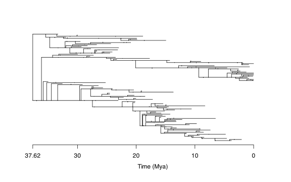
# read our mcc tree
mcc_tree <- read.nexus.buddPhylo(paste0(out_dir, "srfbd_first_mcc.nex"))

You can get some quick details about a buddPhylo object with the print function.

# how many speciation events, how many SAs, and the first 
# few species, with the species that generated them
print(mcc_tree)

## 
## Budding phylogenetic tree with 101 budding speciation nodes and 198 occurrences for 121 species, of which 102 are tips and 19 are sampled ancestors. 
## Species names:
## [1] "Hesperocyon_gregarius"    "Prohesperocyon_wilsoni"   "Otarocyon_macdonaldi"     "Mesocyon_temnodon"       
## [5] "Hesperocyon_coloradensis" "Osbornodon_renjiei"      
## 
## Names of progenitor taxa:
## [1] NA                      NA                      NA                      NA                     
## [5] NA                      "Hesperocyon_gregarius"
## 
## 
## For more details on vector y, try buddPhylo$y, with y one of:
## lineage taxon orientation length name range rate height_mean height_median posterior height_95%_HPD_min height_95%_HPD_max height_range_min height_range_max parent type y_coord x_coord x_par y_par extant

Now let’s investigate some interesting aspects of our MCC tree, and use paleobuddy to write functions to explore that.

First, consider the grey wolf (Canis lupus). I’m sure that’s a lot of reader’s favorite dog. Because this tree explores morphology only, we see the dire wolf species complex (Aenocyon dirus and Canis (Aenocyon) armbrusteri) being recovered very close to lupus (see Perri et al. (2021) and Gedman et al. (2025) for an idea of what happens when we add dire wolf DNA into the mix).

How often does this configuration (dirus-armbrusteri descending from within the lupus range) show up in our posterior sample of trees? We will write a custom function, using a number of paleobuddy functions:

• is.monophyletic.buddPhylo takes a buddPhylo and a list of tips (including the first or last tags), and returns a logical on whether that list of tips is monophyletic in the tree.
• getMRCA.buddPhylo takes the same arguments, and returns the name field of the node that represents the most recent common ancestor (MRCA) of the tips in question.
• getDescendants.buddPhylo takes a buddPhylo and node name, and returns all tips that descend from that node.
• getChildren.buddPhylo takes the same arguments, and returns only the immediate children of the node in question. If the node is a speciation node, the children are names ancestor and descendant to identify the orientation. If it is a sampled ancestor node, the children are named sampAnc and lineage. And if it is a tip, the return is NULL.

# function to check how often a clade is descended
# from within a species's range
direct_descendant <- function(trees, clade, species, lineage = FALSE) {
  sum(unlist(lapply(trees, function(x) {
    # check if clade is monophyletic, if not then this is already not true
    if (!is.monophyletic.buddPhylo(x, clade, 
                                   excludeSampAnc = FALSE)) return(FALSE)
    
    # get the full clade (clade + last occurrence of species)
    full_clade <- sort(c(clade, paste0(species, "_last")))
    
    # if we want to check if the *lineage* of that species generated the
    # clade, we also allow for the budding to be not from within the range
    if (lineage) full_clade <- sort(c(full_clade, paste0(species, "_first")))
    
    # get the node that is the MRCA of clade+last occurrence of species
    mrca <- getMRCA.buddPhylo(x, full_clade)
    
    # find the descendants of this mrca
    desc <- sort(getDescendants.buddPhylo(x, mrca))
    
    # and check if this is exactly equal 
    # to the clade+last occurrence of species
    res <- identical(desc, full_clade)
    
    # if lineage is true, we also need to check that clade is 
    # the descendant child (if not, it must be since it's within the range)
    if (lineage) {
      # get the MRCA of just the clade
      mrca_clade <- getMRCA.buddPhylo(x, clade)
      
      # check that this is the "descendant" member of the children of the MRCA
      res <- res &&
        mrca_clade == getChildren.buddPhylo(x, mrca)[2]
    }
    
    # return
    return(res)
  }))) / length(trees)
}

This function then checks, for each tree, whether the clade is monophyletic, and whether the clade is budding off of directly from the range of species. Optionally (using the lineage argument) we can check whether the clade buds off the lineage leading to the range of that species, instead of within the range itself. These are two distinct, but similar, biological scenarios. Let’s check what the case is for the lupus-armbrusteri-dirus complex.

# define the clade
clade <- c("Aenocyon_dirus_first", "Aenocyon_dirus_last",
           "Canis_armbrusteri_first", "Canis_armbrusteri_last")

# and species
species <- "Canis_lupus"

print(paste0("Proportion of trees where clade buds off of species's range: ",
             direct_descendant(trees, clade, species)))

## [1] "Proportion of trees where clade buds off of species's range: 0.275948103792415"

print(paste0("Proportion of trees where clade buds off of species's lineage: ",
             direct_descendant(trees, clade, species, TRUE)))

## [1] "Proportion of trees where clade buds off of species's lineage: 0.142714570858283"

If you check the node comments of the speciation node in question in our MCC tree (hover the mouse over the branch leading to that node), you will likely see a value that is the sum of those two for the posterior probability of that clade (for my tree, it is posterior = 0.41). That’s because that posterior calculation considers both of these configurations. This is a reasonably low posterior probability, which likely indicates that the data are not extremely uncertain.

We can also ask questions about the higher level topology. For example, the ancient canid Hesperocyon gregarius appears as the oldest species in our MCC tree. All other lineages are budding off of its range. This matches the expert consensus, which is that Hesperocyon, a member of the Hesperocyoninae subfamily, generated the other canid subfamilies, Borophaginae and Caninae. We can check how often this happens in our tree sample fairly easily.

# vector to hold all tips
all_tips <- unique(mcc_tree$lineage)
all_tips <- all_tips[!is.na(all_tips)]

# minor modifications to remove each occurrence of gregarius from all_tips
all_but_hg1 <- all_tips[all_tips != "Hesperocyon_gregarius_first"]
all_but_hg <- all_but_hg1[all_but_hg1 != "Hesperocyon_gregarius_last"]

# function to check which percentage of our tree 
# sample has certain clade as monophyletic
prop_monophyletic <- function(trees, clade) {
  sum(unlist(lapply(trees, function(x)
    is.monophyletic.buddPhylo(x, clade, excludeSampAnc = FALSE)))) / length(trees)
}

# let's check it for those two clades
print(paste0("Proportion of trees where all but H_gregarius_first is monophyletic: ",
             prop_monophyletic(trees, all_but_hg1)))

## [1] "Proportion of trees where all but H_gregarius_first is monophyletic: 0.405189620758483"

print(paste0("Proportion of trees where all but H_gregarius is monophyletic: ",
             prop_monophyletic(trees, all_but_hg)))

## [1] "Proportion of trees where all but H_gregarius is monophyletic: 0.0114770459081836"

For my tree sample, the first value was around 0.41, and the second 0.01. One important thing to note here is that SR trees always have the stratigraphic range of a species unbroken. Because of that, for every tree in our sample with the clade excluding hesperocyon_gregarius_first as monophyletic, there are only two possible configurations they could take:

• The entire Hesperocyon gregarius SR is a sampled ancestor to the rest of Canidae. This would mean that the clade excluding both gregarius occurrences would be monophyletic, which as we saw happens in 1% of our trees.
• All other canid lineages bud off the range of gregarius, as we see in the MCC tree. Because this is the only other option, we can infer that it happens in around 40% of trees in our sample.

Our results therefore weakly support the expert consensus, i.e. H. gregarius having generated the rest of Canidae, another reminder that these data might not be enough to make strong assertions. You can investigate further what might be the first diverging lineage (e.g. try doing the same procedure as above but with Prohesperocyon_wilsoni_first as the excluded tip), and you will find that this is the most likely configuration, even with such a low posterior probability. Still, this is a great example to illustrate the power of SR trees: how easy was it to test such a fundamental hypothesis about the evolutionary history of Canidae?

We could also of course check divergence-time estimates for clades we are interested in. Since budding trees don’t have that much extra to say about divergence times, I will just give one quick example so we can check how to extract this information from buddPhylo objects. Let’s check the distribution of the time at which the first diverging Canidae lineage buds off the range of Hesperocyon gregarius, in the 40% of trees where that happens.

# extract the divergence times
div_times <- unlist(lapply(trees, function(x) {
  # check if all_but_hg1 is monophyletic--if not we don't want this tree
  if (is.monophyletic.buddPhylo(x, all_but_hg1, excludeSampAnc = FALSE)) {
    # get the time 
    return(node.time.buddPhylo(x, getMRCA.buddPhylo(x, all_but_hg1)))
  } else {
    return(NA)
  }
}))

# plot it
hist(div_times,
     main = "Divergence time distribution for Canidae\\H_gregarius_first",
     xlab = "Time (mya)")

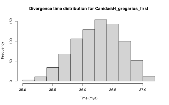
We quickly checked the time of the node representing the MRCA of the clade excluding hesperocyon_gregarius_first with the node.time.buddPhylo function. It seems like most of these trees have that first diverging clade budding off the range of gregarius within a pretty tight 2my interval. It would take a little more defining variables, but we could repeat this analysis to e.g. plot the divergence time between the grey wolf (Canis lupus) and the coyote (Canis latrans), which might give you some information about the timing of the reintroduction of wolf-like canids to North America. Because of the extra information in SR trees, you could even check specifically whether the distribution of divergence times of a clade change when the clade switches orientation. World’s your oyster!

A more detailed analysis of the topology and divergence times of our posterior sample would of course require a much more involved exploration of all the clades in each of the trees, their orientations/sampled ancestor MRCA, and their relative frequencies. Maybe in the future I will write a move involved tutorial about this, but for now I will just mention another paleobuddy function that can aid in that task.

clades <- extract.clades(mcc_tree, 
                         considerSAs = TRUE, considerOrientation = TRUE)
# this generates a total of 197 clades, i.e. length(all_tips) - 1

# check a few clades to understand the formatting
clades[[100]]

## [1] "Cynarctus_crucidens_first, Cynarctus_crucidens_last, Cynarctus_galushai_first, Cynarctus_marylandica_first, Cynarctus_saxatilis_first, Cynarctus_voorhiesi_first\001ANC:Cynarctus_galushai_first; Cynarctus_marylandica_first"

clades[[140]]

## [1] "Aelurodon_asthenostylus_first, Aelurodon_asthenostylus_last, Aelurodon_ferox_first, Aelurodon_ferox_last, Aelurodon_mcgrewi_first, Aelurodon_stirtoni_first, Aelurodon_stirtoni_last, Aelurodon_taxoides_first, Aelurodon_taxoides_last\001SA:Aelurodon_asthenostylus_first"

By default, extract.clades just returns a (sorted) list of strings laying out the clades implied by the tree in the first argument, with tip names separated by commas. You can use the two arguments considerSAs and considerOrientation to get more information on each of these clades. If the former is true, each clade defined by a sampled ancestor node will have the name of the SA species after the \001SA: tag. If the latter is true, each clade defined by a speciation node will have the subset of tips that represent the ancestor side of the budding speciation after the \001ANC: tag. You can therefore use this function to easily list clades contained in each tree, including their orientation and sampled ancestors, to aggregate information about the clades supported in your posterior sample.

Conclusion

In this tutorial, we worked on writing scripts to run SRFBD analyses in BEAST2, and processing the results with paleobuddy. We covered how to write the BEAST2 scripts using my custom R scripts, the basics of assessing convergence for your analyses, and some simple ways to analyze the resulting estimates for parameter values and tree topology.

The stratigraphic-range fossilized birth-death model is a very exciting and powerful model, but it is also highly technical and difficult to use because of the xml setup. I hope I’ve provided you with enough information to apply the model to your own data, and I’m planning to expand this tutorial in the future to help further. Please feel free to contact me if anything was confusing, if I can further help you get an analysis working, or if you have any tips on making this tutorial better. Thank you for reading!

References

Gedman, Gregory L., Kathleen Morrill Pirovich, Jonas Oppenheimer, Chaz Hyseni, Molly Cassatt-Johnstone, Nicolas Alexandre, William Troy, Chris Chao, Olivier Fedrigo, Savannah J. Hoyt, Patrick G. S. Grady, Sam Sacco, William Seligmann, Ayusman Dash, Mithil Chokshi, Laura Knecht, James B. Papizan, Tyler Miyawaki, Sven Bocklandt, James Kelher, Sara Ord, Audrey T. Lin, Brandon R. Peecook, Angela Perri, Mikkel-Holger S. Sinding, Greger Larson, Julie Meachen, Love Dalén, Bridgett vonHoldt, M. Thomas P. Gilbert, Christopher E. Mason, Rachel J. O’Neill, Elinor K. Karlsson, Brandi L. Cantarel, George R. R. Martin, George Church, Ben Lamm and Beth Shapiro. 2025. On the ancestry and evolution of the extinct dire wolf. bioRxiv. https://doi.org/10.1101/2025.04.09.647074.
Heath, T. A., J. P. Huelsenbeck and T. Stadler. 2014. The fossilized birth-death process for coherent calibration of divergence-time estimates. Proceedings of the National Academy of Sciences 111 (29): E2957–E2966. https://doi.org/10.1073/pnas.1319091111.
Lewis, Paul. 2001. A Likelihood Approach to Estimating Phylogeny from Discrete Morphological Character Data. Systematic biology 50: 913–25. https://doi.org/10.1080/106351501753462876.
Perri, Angela R., Kieren J. Mitchell, Alice Mouton, Sandra Álvarez-Carretero, Ardern Hulme-Beaman, James Haile, Alexandra Jamieson, Julie Meachen, Audrey T. Lin, Blaine W. Schubert, Carly Ameen, Ekaterina E. Antipina, Pere Bover, Selina Brace, Alberto Carmagnini, Christian Carøe, Jose A. Samaniego Castruita, James C. Chatters, Keith Dobney, Mario dos Reis, Allowen Evin, Philippe Gaubert, Shyam Gopalakrishnan, Graham Gower, Holly Heiniger, Kristofer M. Helgen, Josh Kapp, Pavel A. Kosintsev, Anna Linderholm, Andrew T. Ozga, Samantha Presslee, Alexander T. Salis, Nedda F. Saremi, Colin Shew, Katherine Skerry, Dmitry E. Taranenko, Mary Thompson, Mikhail V. Sablin, Yaroslav V. Kuzmin, Matthew J. Collins, Mikkel-Holger S. Sinding, M. Thomas P. Gilbert, Anne C. Stone, Beth Shapiro, Blaire Van Valkenburgh, Robert K. Wayne, Greger Larson, Alan Cooper and Laurent A. F. Frantz. 2021. Dire wolves were the last of an ancient New World canid lineage. Nature 591 (7848, 7848): 87–91. https://doi.org/10.1038/s41586-020-03082-x.
Slater, Graham J. 2015. Iterative adaptive radiations of fossil canids show no evidence for diversity-dependent trait evolution. Proceedings of the National Academy of Sciences 112 (16): 4897–4902. https://doi.org/10.1073/pnas.1403666111.
Stadler, Tanja. 2010. Sampling-through-time in birth-death trees. Journal of Theoretical Biology 267 (3): 396–404. https://doi.org/10.1016/j.jtbi.2010.09.010.
Stadler, Tanja, Alexandra Gavryushkina, Rachel C. M. Warnock, Alexei J. Drummond and Tracy A. Heath. 2018. The fossilized birth-death model for the analysis of stratigraphic range data under different speciation modes. Journal of Theoretical Biology 447: 41–55. https://doi.org/10.1016/j.jtbi.2018.03.005.
Stolz, Ugnė, Alexandra Gavryushkina, Timothy G. Vaughan, Tanja Stadler and Bethany J. Allen. 2025. Enhancing Evolutionary Timelines: The Impact of Stratigraphic Range Information on Phylogenetic Inference. https://doi.org/10.1101/2025.04.17.649084.